Analyzing time-to-event data, focusing on the duration until an event of interest occurs.
General Principles
Survival analysis studies the time until an event of interest (e.g., death, recovery, information acquisition) occurs. When analyzing binary survival outcomes (e.g., alive or dead), we can use models such as Cox proportional hazards to evaluate the effect of predictors on survival probabilities.
Key concepts include:
Hazard Function: The instantaneous risk of the event occurring at a given time.
Survival Function: The probability of surviving until a given time.
Covariates: Variables (e.g., age, treatment) that may affect survival probabilities.
Baseline Hazard: The hazard when all covariates are zero, which forms the reference for comparing different conditions.
Considerations
Note
In survival analysis:
The baseline hazard can follow distributions like Exponential, Weibull, or Gompertz, depending on the data.
Censoring (when the event is not observed for some subjects) must be accounted for in the likelihood function. Proper handling is essential for unbiased results.
Bayesian survival models allow flexible handling of time-dependent covariates, random effects, and incorporate uncertainty more naturally than Frequentist methods.
Example
Here’s an example of a Bayesian survival analysis using the BayesForge (BF) package. The data come from a clinical trial of mastectomy for breast cancer. The goal is to estimate the effect of the metastasized covariate, coded as 0 (no metastasis) and 1 (metastasis), on the survival outcome event for each patient. Time is continuous and censoring is indicated by the event variable.
Data and discrete-time setup (shared by both approaches below).
Code
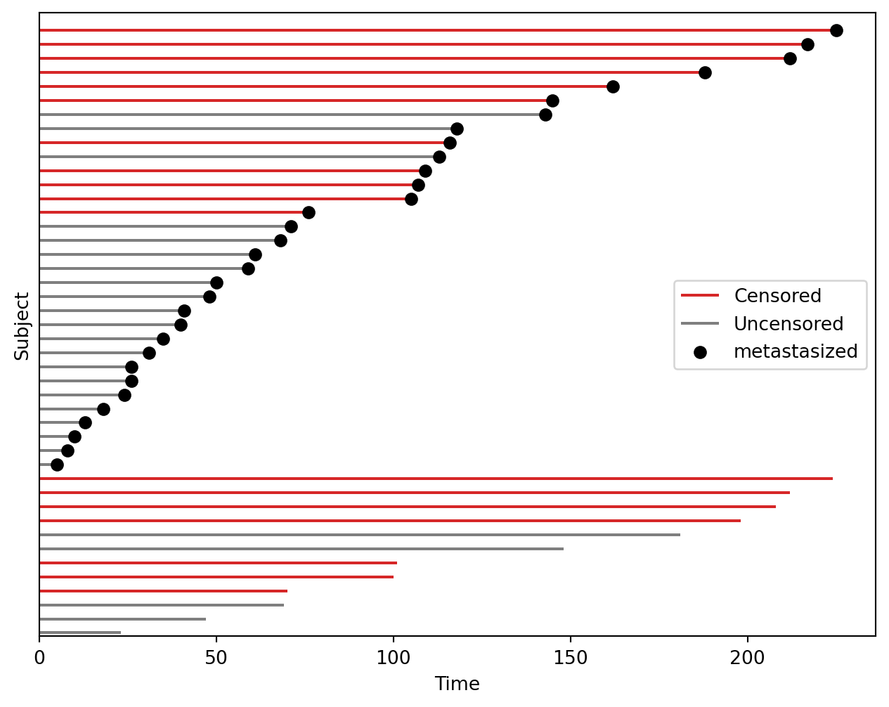
from BayesForge import bfimport numpy as npimport jax.numpy as jnpm = bf(platform='cpu')# --- Data ------------------------------------------------------------# Mastectomy trial. Columns: `time` = follow-up length, `event` = 1 if# death was observed, 0 if the patient was censored (left the study# event-free), `metastasized` = "yes"/"no".data_path = m.load.mastectomy(only_path=True)m.data(data_path, sep=',')m.df.metastasized = (m.df.metastasized.values =="yes").astype(np.int64)# --- Piecewise-constant hazard setup -------------------------------# Cut follow-up time into fixed intervals of length 3. For every# (subject, interval) this builds two matrices:# death[i, k] -> 1 if subject i had the event in interval k# exposure[i, k] -> time subject i spent at risk in interval k# Censoring is encoded here: after a subject leaves (event OR censoring)# its exposure is 0 in every later interval, so it stops contributing# to the likelihood without being counted as a death.m.models.survival.import_time_even(m.df.time.values, m.df.event.values, interval_length=3)# Register `metastasized` as a patient-level (time-invariant) covariate.m.models.survival.import_covF(m.df.metastasized.values, ["metastasized"])# --- Censoring plot -----------------------------------------------# One horizontal line per subject = observed follow-up. Red = censored# (event never seen), grey = event observed, black dot = metastasized.# Reading it: metastasized patients tend to have shorter lines ending# in an event -> a first visual clue of a positive hazard effect.m.models.survival.plot_censoring(cov="metastasized")
bf v 0.0.48 package loaded
jax.local_device_count 32
------------------------------------------------------------------------------
Survival concern 44 individuals in 76 intervals.
26.0 individuals experienced the event.
------------------------------------------------------------------------------
Covariates imported: ['metastasized']
Surv object now has 1 covariates: ['metastasized']
The full model written out, to show every prior and the likelihood.
Code
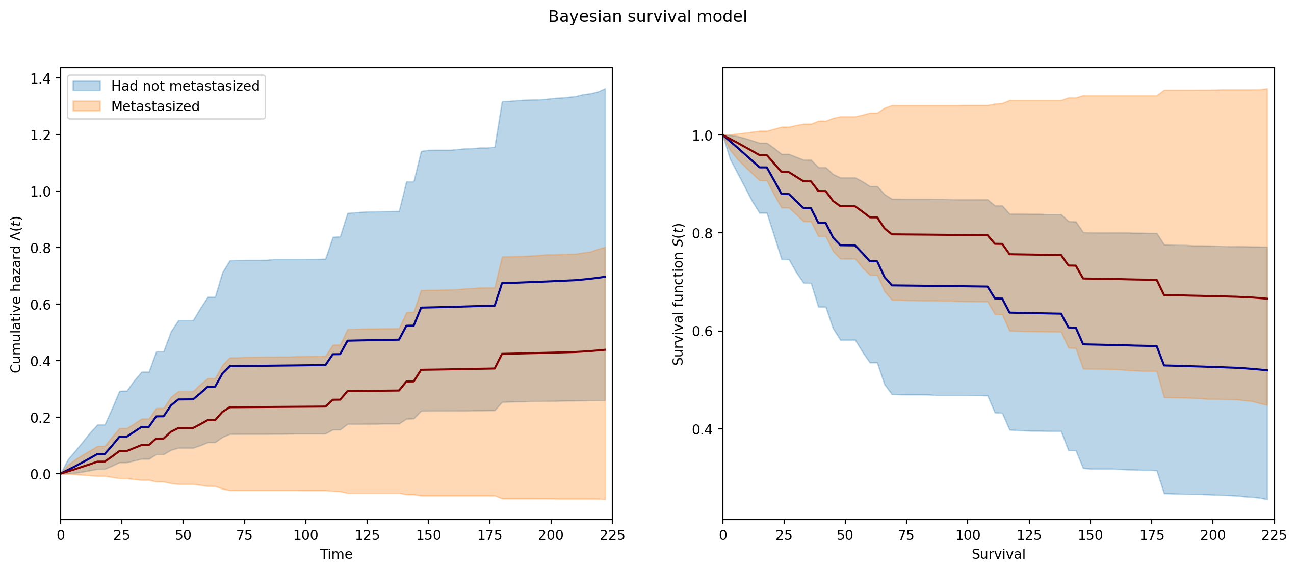
def model(death, cov, exposure, censoring=None):# --- Priors ---------------------------------------------------# Baseline hazard: ONE positive rate per time interval. A# Gamma(0.01, 0.01) prior is almost flat on (0, inf), so the shape# of the hazard over time is driven by the data, not by a# parametric family (Weibull, Gompertz, ...). This is what makes# the model semi-parametric. lambda0 = m.dist.gamma(0.01, 0.01, shape=(exposure.shape[1],), name="Baseline_rate")# Covariate effect on the LOG hazard. Normal(0, 10) is weakly# informative: centred on 0 (no effect) but wide enough to let the# data move it. exp(beta) is the hazard ratio for metastasized. beta = m.dist.normal(0, 10, shape=(1,), name="Hazard_rate_metastasized")# --- Likelihood -------------------------------------------------# Proportional hazards: lambda[i,k] = lambda0[k] * exp(beta * x_i).# Expected event count mu = lambda * exposure; the 0/1 event# indicator is modelled as Poisson (equivalent to the piecewise# exponential survival likelihood). lambda_ = jnp.exp(beta * cov.squeeze())[:, None] * lambda0[None, :] mu = exposure * lambda_ m.dist.poisson(mu + jnp.finfo(mu.dtype).tiny, obs=death)# 4 chains and target_accept_prob=0.99: the many near-empty late# baseline intervals make the geometry awkward, so a higher acceptance# target keeps the step size small enough to mix well.m.fit(model, num_samples=2000, num_warmup=2000, num_chains=4, target_accept_prob=0.99, progress_bar=False)print(m.summary())# Posterior cumulative hazard and survival curves, by covariate group.m.models.survival.plot_surv(beta="Hazard_rate_metastasized")
(<Figure size 1536x576 with 2 Axes>,
 (<Axes: xlabel='Time', ylabel='Cumulative hazard $\\Lambda(t)$'>,
  <Axes: xlabel='Survival', ylabel='Survival function $S(t)$'>))
Same model, assembled by BF from the imported survival object. Priors are attributes you can override before fit.
Code
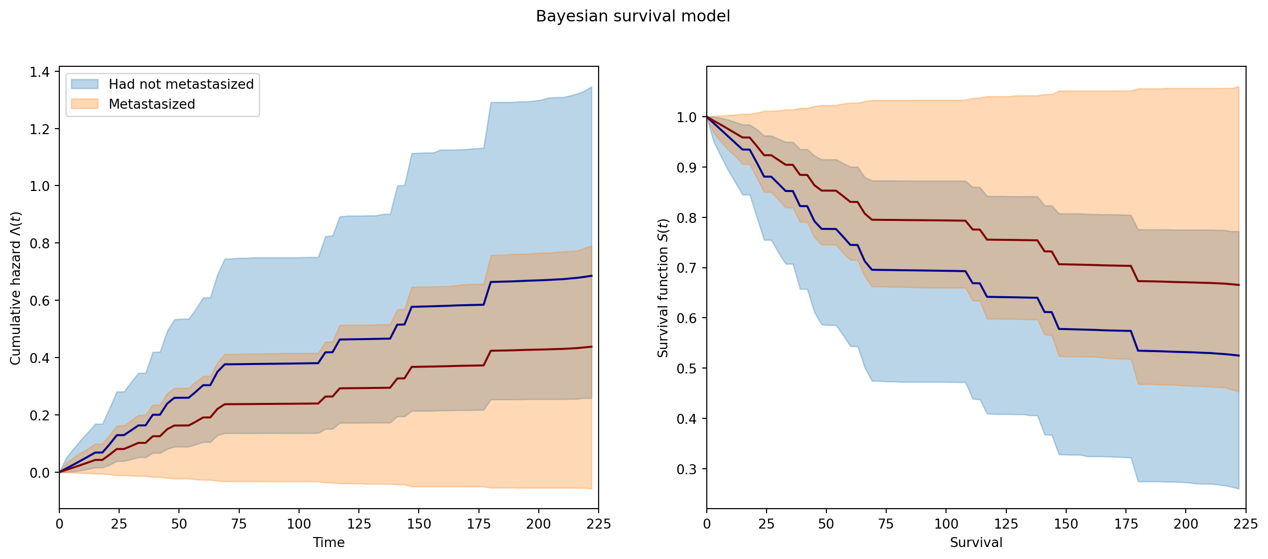
# Optional: change the default priors (shown with their defaults).m.models.survival.baseline_rate_prior = (0.01, 0.01) # Gamma(conc, rate)m.models.survival.hazard_rate_prior_scale =10.0# Normal(0, scale)m.fit(m.models.survival.model)print(m.summary())m.models.survival.plot_surv(beta="Hazard_rate_metastasized")
⚠️This function is still in development. Use it with caution. ⚠️
⚠️This function is still in development. Use it with caution. ⚠️
⚠️This function is still in development. Use it with caution. ⚠️
⚠️This function is still in development. Use it with caution. ⚠️
⚠️This function is still in development. Use it with caution. ⚠️
⚠️This function is still in development. Use it with caution. ⚠️
⚠️This function is still in development. Use it with caution. ⚠️
⚠️This function is still in development. Use it with caution. ⚠️
                         mean      sd  hdi_5.5%  hdi_94.5%  mcse_mean  \
Baseline_rate[0]         0.00    0.00      0.00       0.00       0.00
Baseline_rate[1]         0.00    0.00      0.00       0.01       0.00
Baseline_rate[2]         0.00    0.00      0.00       0.01       0.00
Baseline_rate[3]         0.00    0.01      0.00       0.01       0.00
Baseline_rate[4]         0.00    0.01      0.00       0.01       0.00
...                       ...     ...       ...        ...        ...
log_Baseline_rate[71] -100.21   95.99   -219.87      -1.79       3.13
log_Baseline_rate[72] -100.90   96.95   -220.47      -2.42       3.09
log_Baseline_rate[73] -100.25  100.58   -224.29      -1.31       3.96
log_Baseline_rate[74] -107.25  108.60   -236.36      -1.74       4.72
log_Baseline_rate[75] -100.22  103.53   -229.62       5.43       3.71

                       mcse_sd  ess_bulk  ess_tail  r_hat
Baseline_rate[0]          0.00   1030.11    925.87   1.01
Baseline_rate[1]          0.00   1830.03   1647.97   1.00
Baseline_rate[2]          0.00   1678.37   1391.43   1.00
Baseline_rate[3]          0.00   2482.44   1769.31   1.00
Baseline_rate[4]          0.00   2014.18   1680.21   1.00
...                        ...       ...       ...    ...
log_Baseline_rate[71]     4.95   1246.09   1176.13   1.00
log_Baseline_rate[72]     4.08   1259.81   1210.91   1.00
log_Baseline_rate[73]     5.75    914.15    696.20   1.00
log_Baseline_rate[74]     7.01    822.05    616.83   1.00
log_Baseline_rate[75]     4.48    944.59    995.43   1.00

[153 rows x 9 columns]
(<Figure size 1536x576 with 2 Axes>,
 (<Axes: xlabel='Time', ylabel='Cumulative hazard $\\Lambda(t)$'>,
  <Axes: xlabel='Survival', ylabel='Survival function $S(t)$'>))
Survival plot. Left: posterior cumulative hazard \Lambda(t) = \sum_k \lambda_0^{(k)}\Delta_k per covariate group; right: the implied survival S(t) = e^{-\Lambda(t)}. Solid line = posterior mean, shaded band = 94% credible interval, blue = not metastasized, orange = metastasized. The size and direction of the effect are read from \beta (equivalently the hazard ratio e^{\beta}) in m.summary(); here \beta > 0, i.e. metastasis raises the hazard.
Mathematical Details
Bayesian formulation
The BF survival model uses a piecewise-constant hazard (Poisson counting-process) approach. The continuous follow-up time is divided into K fixed intervals of length \Delta. Each subject i in interval k contributes:
N_{ik} is the number of events (0 or 1) recorded for subject i in interval k.
e_{ik} is the exposure (time at risk) for subject i in interval k. It equals \Delta if the subject is fully observed in the interval, a fractional value if the subject exits (via event or censoring) mid-interval, and 0 if the subject has already left the risk set. This term is the mechanism that handles censoring: once a subject is censored or experiences the event, their exposure drops to 0 in all subsequent intervals.
\mu_{ik} = \lambda_{ik} \cdot e_{ik} is the expected number of events, i.e., the hazard rate scaled by time at risk.
\lambda_{ik} is the hazard rate for subject i in interval k, decomposed into a baseline hazard\lambda_0^{(k)} and a covariate-specific multiplicative shift.
\lambda_0^{(k)} is the baseline hazard in interval k, constant within each interval but free to vary across intervals. This gives the model non-parametric flexibility over time. A Gamma(0.01, 0.01) prior (BF default m.models.survival.baseline_rate_prior) places minimal information on the baseline hazard; on the numpyro backend it is sampled in log space for stability.
X_i is the vector of covariates for subject i.
\beta is the vector of regression coefficients. The coefficient \exp(\beta) gives the hazard ratio: the multiplicative change in hazard for a unit increase in the corresponding covariate. A weakly informative Normal(0, 10) prior is centred on “no effect” but wide on the log-hazard scale. It is the BF default (m.models.survival.hazard_rate_prior_scale).
Survival and hazard functions
From the posterior samples of \lambda_0^{(k)} and \beta, two key quantities can be derived:
Where \Delta_k is the width of interval k. ## Reference(s) https://en.wikipedia.org/wiki/Proportional_hazards_model https://www.mathworks.com/help/stats/cox-proportional-hazard-regression.html https://www.pymc.io/projects/examples/en/latest/survival_analysis/survival_analysis.html https://vflores-io.github.io/posts/20240924_numpyro_logreg_surv_analysis/np01_logreg_surv_analysis/